Have you ever wondered how generative AI produces strikingly realistic images? The secret lies in Generative Adversarial Networks (GANs)—a groundbreaking AI model introduced by Ian Goodfellow in 2014.a
GAN image generation has revolutionized artificial intelligence by producing high-quality images from random noise.
It’s no surprise that Yann LeCun, Meta’s AI research director, calls adversarial training “the most interesting idea in the last 10 years in machine learning.”
In this blog, we’ll break down the core elements of GAN architecture, including the generator and discriminator, and show you how these networks collaborate to generate images. We’ll also guide you through an example to help you understand how GANs work in practice. Let’s dive in.
What is Generative Adversarial Networks (GAN)?
GAN is an algorithm that uses two neural networks, Generator G and Discriminator D. The two networks compete against one another (hence the term ‘adversarial’).
The generator creates synthetic data, while the Discriminator tries to distinguish between the generated data and real data. This leads to creating highly realistic data that can often pass for real.
Over the past few years, GAN has made significant progress. A remarkable example is an AI-generated portrait that sold for $432,000—an artwork produced by a GAN. GANs power modern AI Image Generation Software listed on Spotsaas, enabling realistic visuals and artwork creation from simple inputs. Impressive, right?
To fully understand GANs, it’s crucial to grasp how the Generator and Discriminator work together.
Generator
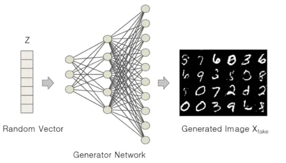
The Generator (G) in GAN is responsible for producing synthetic samples from random inputs, often just a set of noise or values. It acts as the core of the GAN architecture, gradually learning to create highly realistic images as the training progresses.
For example, if you train the imagineart ai image generator on images of cats, it will compute and generate an image that resembles a cat—though the image is entirely synthetic. Each output will be different, as the Generator takes a new random input (called the noise vector) each time, ensuring the creation of diverse images with every run. This process can also be useful for tasks related to image editing, where subtle adjustments or creative variations of existing visuals are needed.
Since the Generator is in constant competition with the Discriminator, it strives to create fake images so realistic that the Discriminator mistakenly classifies them as real.
Discriminator
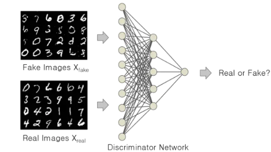
The Discriminator, on the other hand, processes the images created by the Generator and classifies them as either real or fake. It is presented with both the real samples from the training data and the fake image produced by the generator.
Gradually, the Discriminator learns to distinguish between the two samples and offers crucial feedback to the Generator about the quality of the generated samples.
How GAN Works: A Closer look?
The constant confrontation between the Generator and Discriminator results in an iterative learning cycle.
As the training progresses, the Generator becomes better at producing realistic samples, while the Discriminator becomes more adept at distinguishing real data from fake. Over time, this adversarial process leads to the Generator creating samples that look increasingly authentic.
Ideally, the training process must reach an equilibrium, where the Generator produces data and the Discriminator can no longer distinguish between real and synthetic data. At this point, the Discriminator’s accuracy drops to around 50%, meaning it is essentially guessing whether the input is real or fake.
However, reaching this equilibrium can be challenging. Several factors—like the network’s architecture, the choice of hyperparameters, and the complexity of the dataset—can affect training stability. If not balanced properly, the Generator and Discriminator may enter into a loop of oscillating solutions or encounter mode collapse, where the Generator produces limited, repetitive outputs instead of diverse samples.
Additionally, if the Discriminator becomes too powerful early in the training process, it can easily reject the Generator’s outputs. This hampers the Generator’s ability to learn, as it receives little feedback on how to improve its performance in generating realistic data.
Generating Images with GAN
Now that we understand how GANs work, let’s move into the details of how to implement GANs to generate images.
We’d be implementing code on Google collab and we used the TensorFlow library. You can access the full code here.
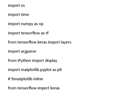
STEP 1: Import the necessary libraries
The relevant libraries must first be loaded.
STEP 2: Load the data and conduct data preprocessing
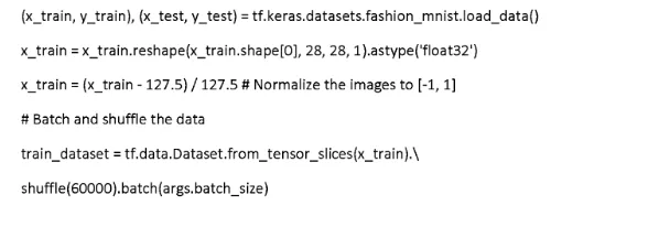
In this example, we load the Fashion MNIST dataset using the ‘tf_keras’ datasets module. We don’t need labels to solve this problem, hence we only make use of the training images, x_train. Next, we reshape the images, and because the data is in unit8 format by default, we cast them to float32.
Our preprocessing also involves normalizing the data from [0, 255] to [-1, 1]. Then we build the TensorFlow input pipeline. Summarily, we feed the ‘tf.data.Dataset.from_tensor_slices’ with the training data, shuffle, and slice it into tensors which allows us to access tensors of defined batch size during training.
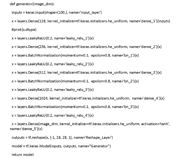
STEP 3: Create the Generator Network
Here, we have fed the generator with a 100-D noise vector which was sampled from a normal distribution. The next thing we do is to define the input layer with the shape (100,). ‘he_uniform’ is the default weight initializer for the linear layers in Tensor Flow.
Then, we use ‘tf.reshape’ to reshape the 784-D tensor to batch sizes 28, 28, and 1, the first parameter being the input tensor and the second being the new shape of the tensor.
We finally pass the generator function’s input and output layer to create the model.
STEP 4: Create the discriminator network
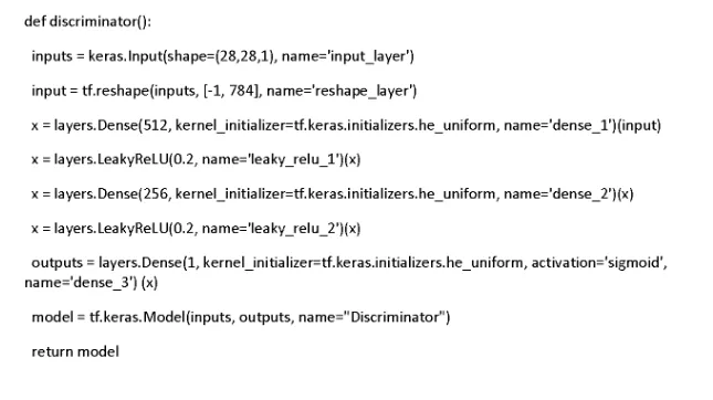
The discriminator is a binary classifier and only has fully connected layers. Because of this, it’s only expecting a tensor of shape (Batch Size, 28, 28, 1). However, the discriminator function only has dense layers, which means we have to reshape the tensor to a vector of shape which is Batch Size, 784. You’d see the sigmoid activation function on the last layer, and what this does is produce the output value between 0 (fake) and 1 (real).
STEP 5: Define the loss function
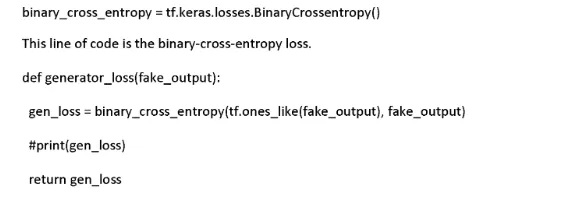
This is the generator’s individual loss
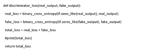
And this is the discriminator’s loss.
STEP 6: Optimize both the generator and discriminator
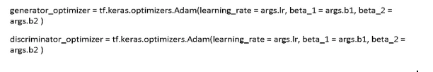
To optimize both the generator and discriminator, we use ‘Adam Optimizer,’ and this takes two arguments which are the learning rate and beta coefficients.
During backpropagation, these arguments compute the running averages of gradients.
The core of the whole GAN training is the ‘train_step’ function. This is because we can combine all the training functions as defined above.
What the ‘@tf.function’ does is compile the train_step function into a TensorFlow graph that we can call. Additionally, it reduces training time.
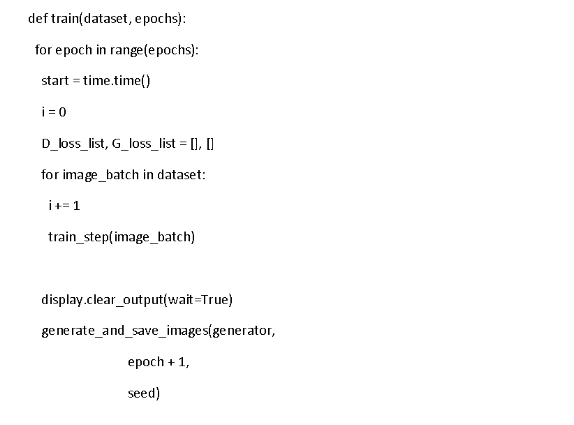
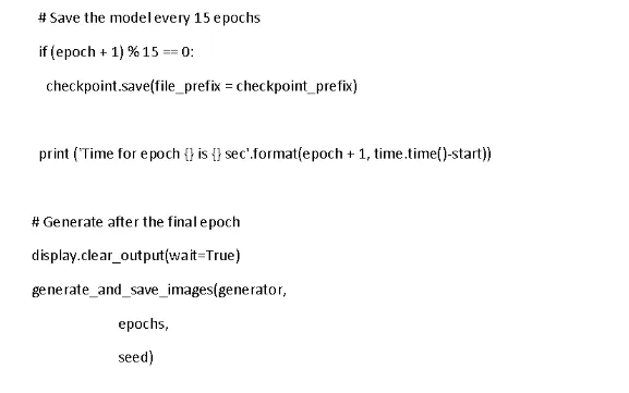
STEP 7: Final Training
Finally, the time has arrived for us to sit and view the magic, but let’s pause for a minute. The function above requires two parameters (training data and number of epochs). When you give it those parameters, you can then proceed to run the program and watch as GAN does its magic.
Unlock the Power of GANs for Your Business with Algoscale
Generative Adversarial Networks are transforming industries by enabling hyper-realistic image generation, synthetic data creation, and next-level AI solutions. At Algoscale, we help businesses harness GANs and other advanced AI models to innovate, scale, and stay competitive. Whether you’re exploring AI-driven creativity, automation, or analytics, our experts can guide you from strategy to implementation.
Get Started with GANs Today
How Can Algoscale Help in Leveraging GANs for your business?
In this article, we have seen what GANs are, how they work, and how you can use them to generate images. We hope you found it useful and we’d like to inform you that if you stay connected with us, we have more in store for you.
No matter where you are in your journey, Algoscale is here to help you succeed in the big data era. As an top data consulting agency, we specialize in leveraging cutting-edge technologies like GANs to create tailored solutions for businesses across industries. Whether you’re looking to apply GANs for innovation, research, or commercial projects, our team is ready to support you every step of the way.